OAE Atlas Dataset - Atlas Calculations

This notebook downloads a curated subset of the Ocean Carbon Dioxide Removal (OAE) Atlas dataset to a local cache using the S3 access helpers in cdr_atlas.py. It also provides quick visual checks and documentation of what is being downloaded.

Dataset hosted on Source Cooperative: https://source.coop/cworthy/oae-efficiency-atlas

Dataset summary¶

The dataset contains results from thousands of CESM ocean alkalinity enhancement simulations.
Files are organized by polygon (region), injection month, and simulation year/month.
Each experiment includes perturbation variables and counterfactual variables (suffix _ALT_CO2).
Polygon masks and efficiency maps are provided as NetCDF files.

Use this notebook to prefetch data in batches to avoid repeated downloads during analysis.

%load_ext autoreload
%autoreload 2

from pathlib import Path

import numpy as np
import xarray as xr
import yaml

import atlas_engine

/global/homes/m/mattlong/.conda/envs/cson-atlas/lib/python3.13/site-packages/pop_tools/__init__.py:4: UserWarning: pkg_resources is deprecated as an API. See https://setuptools.pypa.io/en/latest/pkg_resources.html. The pkg_resources package is slated for removal as early as 2025-11-30. Refrain from using this package or pin to Setuptools<81.
  from pkg_resources import DistributionNotFound, get_distribution

Configuration¶

Choose a polygon ID, injection month, and a set of model years to download. The files follow:

experiments/{polygon_id}/{injection_month}/alk-forcing.{polygon_id}-{injection_year}-{injection_month}.pop.h.{year}-{month}.nc

polygon_id ranges from 000–690 and injection_month is typically 01/04/07/10 for the published experiments. Use n_test to limit the number of files pulled.

Model year 0347 corresponds to the calendar year 1999, thus we need a model_year_offset to align the model calendar with the true calendar year.

batch_size = 50

 # set any to None to download all available
injection_year = 1999
injection_month = 1

# n_test limits the number of files downloaded
n_test = 2

dask_cluster_kwargs = {}

# Parameters
injection_year = 1999
injection_month = 1
n_test = None
dask_cluster_kwargs = {
    "account": "m4632",
    "queue_name": "premium",
    "n_nodes": 1,
    "n_tasks_per_node": 128,
    "wallclock": "06:00:00",
    "scheduler_file": None,
}

Step 1: Identify files to download¶

We first enumerate all expected files for this polygon/time window. This avoids repeated S3 listings during computation.

atlas_data = atlas_engine.datasets["oae-efficiency-map_atlas-v0"]
atlas_data.df

manifest = atlas_data.query(injection_year=injection_year, injection_month=injection_month, n_test=n_test)
manifest

Step 2: Download missing files in batches¶

Downloads happen in batches to reduce overhead and better utilize S3 transfer throughput.

downloaded = atlas_data.ensure_cache(injection_year=injection_year, injection_month=injection_month, n_test=n_test)

print(f"{len(downloaded)} file(s) in cache: {atlas_data.cache_dir}")

124200 file(s) in cache: /pscratch/sd/m/mattlong/atlas_cache

Step 3: Open cached data and inspect variables¶

This uses the cached NetCDF files and avoids any further network transfer.

First, select a downloaded polygon.

polygon_id = atlas_data.query(injection_year=injection_year, injection_month=injection_month, n_test=n_test).polygon_id.unique()[0].item()
polygon_id

0

ds = atlas_data.open_dataset(polygon_id=polygon_id, injection_year=injection_year, injection_month=injection_month, n_test=n_test)
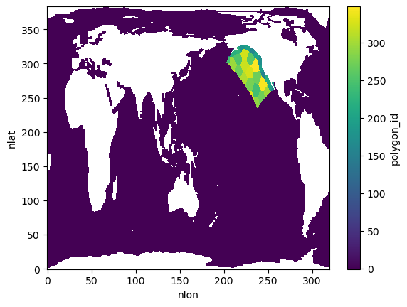
ds

Plot 1: Polygon mask overview¶

The polygon masks dataset defines the spatial regions used in the experiments. This plot previews the polygon IDs on the global grid.

ds_atlas_polygons = atlas_data.get_polygon_masks_dataset()
polygon_ids = ds_atlas_polygons.polygon_id
polygon_ids.plot()

Plot 2: Example FG_CO2 slice¶

The dataset includes FG_CO2 and FG_ALT_CO2 variables (perturbation vs. counterfactual). This plots one slice for the selected polygon and injection date.

injection_date = f"{injection_year:04d}-{injection_month:02d}"

fg_co2 = ds.FG_CO2.sel(
    polygon_id=polygon_id, injection_date=injection_date
).isel(elapsed_time=0)

fg_co2.plot()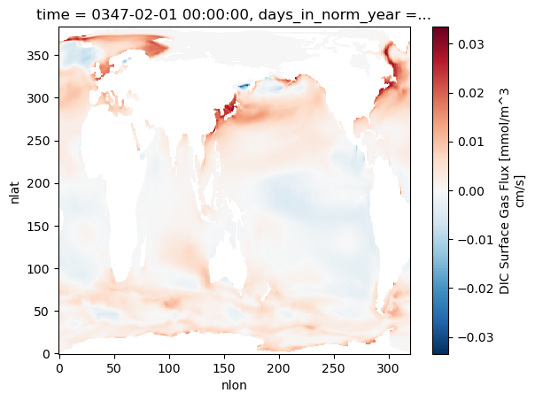

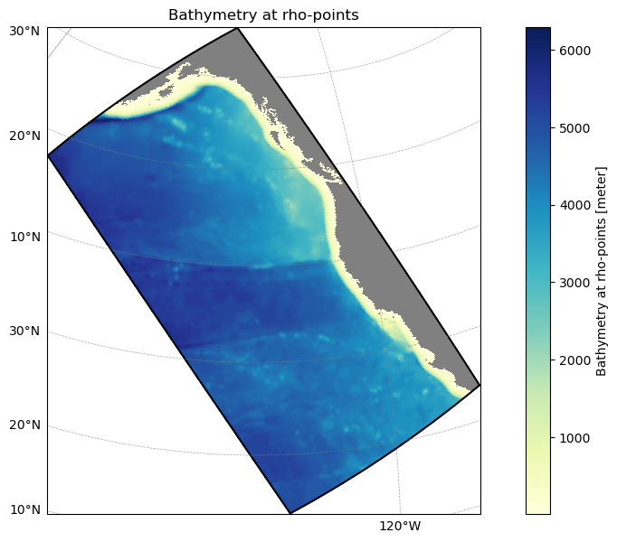
Example 3: Subset to a ROMS-Tools grid¶

Use a ROMS-Tools grid YAML to find which atlas polygons intersect your model domain. This is a lightweight spatial filter that you can use before downloading or integrating data.

from atlas_engine.parsers import load_roms_tools_object

domain_name = "cson_roms-marbl_v0.1_ccs-12km"

# Path to a ROMS-Tools grid YAML
grid_yaml = f"../blueprints/{domain_name}/_grid.yml"
model_grid = load_roms_tools_object(grid_yaml)

model_grid.plot()

# Create AtlasModelGridAnalyzer instance
analyzer = atlas_engine.datasets["oae-efficiency-map_atlas-v0"].analyzer(model_grid)

# Get polygon IDs within model grid boundaries
print(f"Found {len(analyzer.polygon_ids_in_bounds)} unique polygon IDs within model grid boundaries")
print(f"Polygon IDs: {analyzer.polygon_ids_in_bounds[:100]}..." if len(analyzer.polygon_ids_in_bounds) > 100 else f"Polygon IDs: {analyzer.polygon_ids_in_bounds}")

analyzer.polygon_id_mask.plot(vmin=-1, vmax=analyzer.polygon_id_mask.max())

Found 34 unique polygon IDs within model grid boundaries
Polygon IDs: [152. 154. 159. 164. 167. 172. 180. 192. 194. 199. 201. 214. 219. 226.
 243. 244. 250. 259. 269. 270. 271. 276. 289. 290. 295. 299. 306. 320.
 324. 326. 328. 331. 345. 348.]