Tidal gauge–model SSH comparison
This notebook compares Grundartangi tidal gauge sea-level data with the Iceland2 model sea-surface height (zeta).
Gauge data: Load and time-parse the Grundartangi record into an
xarray.Dataset.Model extraction: Load Iceland2 history files, regrid
zeta, and sample the nearest grid point to the gauge.Time series comparison: Plot overlapping SSH time series for a several-month window.
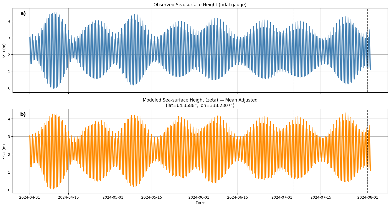
Mean-offset correction: Align model and observed mean sea level and re-plot to focus on tidal and subtidal variability.
This is useful for checking whether the model reproduces tidal amplitude/phase and low-frequency SSH signals at the fjord head.
import subprocess
import os

import netCDF4
import numpy as np
import glob
import time
import matplotlib.pyplot as plt
import copy
import xarray as xr
from datetime import datetime, timedelta
from roms_regrid import *
from celluloid import Camera
import cartopy.crs as ccrs
import seawater as sw
import pandas as pd
/tmp/ipykernel_3502304/2849830013.py:15: UserWarning: The seawater library is deprecated! Please use gsw instead.
import seawater as sw
import pandas as pd
import xarray as xr

# Read file
f='/home/x-uheede/R/HAFRO/Grundartangi_01012024-30122024.xlsx'
grundartangi = pd.read_excel(f, decimal=',')

# Parse time
time = grundartangi['Timabil'].str.strip()
time = pd.to_datetime(time, format="%H:%M\n%d.%m.%Y", dayfirst=True)

# Replace column
grundartangi['time'] = time

# Set time as index (optional but recommended)
grundartangi = grundartangi.set_index('time')

# Convert to xarray
ds = xr.Dataset.from_dataframe(grundartangi)
ds = ds.sortby("time")
ds
Loading...
grundartangiLoading...
plt.plot(ds.time)
model_grid_path="/home/x-uheede/S/Iceland2_MARBL_2024_60m/P_INPUT/Iceland2_grid.nc"
# Grid parameters, only modify these if grid is made in MATLAB
vert_levels=60
theta_s_model=5
theta_b_model=2
hc_model=300
model_data_path="/anvil/scratch/x-uheede/Iceland2_MARBL_2024_60m/Iceland2_MARBL_2024_his.20240?????????.nc"
from roms_tools import Grid, ROMSOutput
grid = Grid.from_file(
    model_grid_path
)
#Only run this cell if grid is made in MATLAB
#grid.update_vertical_coordinate(N=vert_levels, theta_s=theta_s_model, theta_b=theta_b_model, hc=hc_model, verbose=False)
import xarray as xr
import numpy as np
target_depth_levels=[1,2,3,4,5,7,9,10,12,14,15,16,18,20,26,30,36,40,50,80] # Specify depth levels of interest
# Load ROMS output using your pattern
roms_output = ROMSOutput(
grid=grid,
path=[
model_data_path,
],
use_dask=True,
)
ds_model = roms_output.regrid(var_names=["zeta"])ds_model.load()Loading...
# Identify duplicates in the time coordinate
duplicates = ds_model['time'].to_index().duplicated()

# Drop duplicate time steps
ds_model_unique = ds_model.sel(time=~duplicates)
plt.figure(figsize=(14,5))
plt.plot(ds["time"].sel(time=slice('2024-06-01','2024-07-31')), ds["Flodtafla (m)"].sel(time=slice('2024-06-01','2024-07-31')), color="steelblue")
plt.title("Sea Surface Height (Flodtafla) — Timeseries")
plt.xlabel("Time")
plt.ylabel("Sea Surface Height (m)")
plt.grid(True)
plt.tight_layout()
plt.show()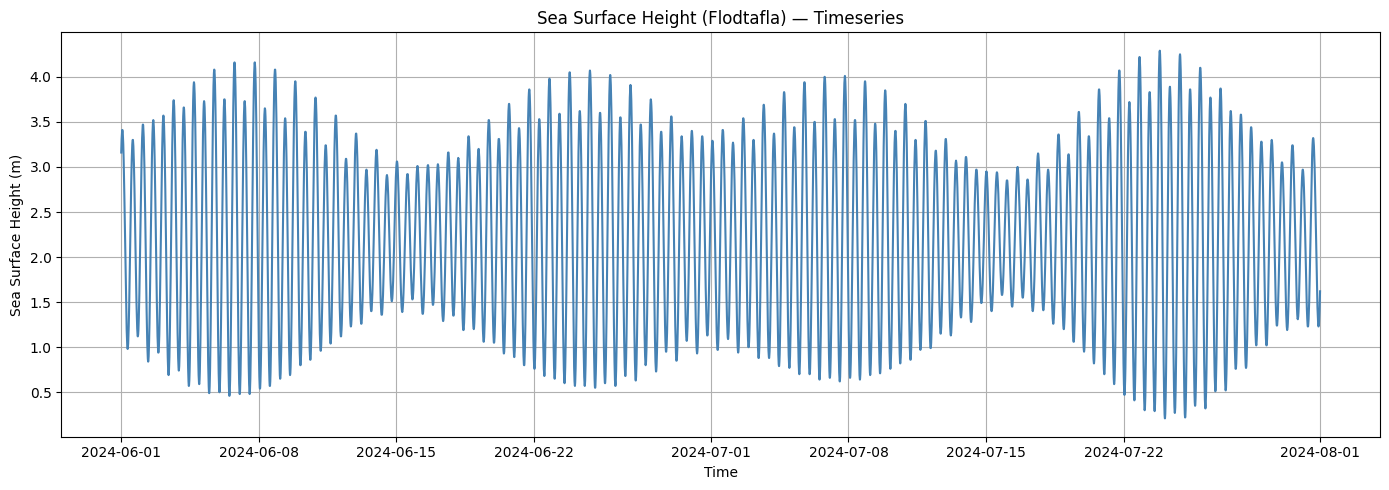
import matplotlib.pyplot as plt
import pandas as pd

line1 = pd.to_datetime("2024-07-05")
line2 = pd.to_datetime("2024-08-01")
# 64.358799°N 21.769334°W

# Convert lon_W to 0–360 range
lon_target = 360 - 21.769334   # = 338.230666
lat_target = 64.358799

# Select nearest model grid point for zeta
zeta_point = ds_model_unique["zeta"].sel(
    lon=lon_target,
    lat=lat_target,
    method="nearest"
)

# Select same time window
t0, t1 = "2024-04-01", "2024-08-01"

ssh_obs = ds["Flodtafla (m)"].sel(time=slice(t0, t1))
ssh_time = ds["time"].sel(time=slice(t0, t1))

zeta_mod = zeta_point.sel(time=slice(t0, t1))


# --------------------------------------------------------
# Compute mean SSH for observations and model
# --------------------------------------------------------
mean_obs = float(ssh_obs.mean())
mean_mod = float(zeta_mod.mean())

# Compute offset so means match
offset = mean_obs - mean_mod

print("Mean observed SSH  :", mean_obs)
print("Mean modeled SSH   :", mean_mod)
print("Vertical offset Δ  :", offset)

# Apply correction
zeta_mod_corrected = zeta_mod + offset

# --------------------------------------------------------
# Plot 2-panel figure
# --------------------------------------------------------
fig, (ax1, ax2) = plt.subplots(
    2, 1, figsize=(15, 8), sharex=True,
    gridspec_kw={"height_ratios": [1, 1]}
)

# -------------------------------------
# Panel 1 — Observed Flodtafla
# -------------------------------------
ax1.plot(ssh_time, ssh_obs, color="steelblue")
ax1.set_title("Observed Sea-surface Height (tidal gauge)")
ax1.set_ylabel("SSH (m)")
ax1.grid(True)

# Add panel label
ax1.text(
    0.02, 0.92, "a)",
    transform=ax1.transAxes,
    fontsize=14,
    fontweight="bold"
)
ax1.axvline(line1, color="black", linestyle="--", linewidth=1.5)
ax1.axvline(line2, color="black", linestyle="--", linewidth=1.5)

# -------------------------------------
# Panel 2 — Modeled zeta (mean-corrected)
# -------------------------------------
ax2.plot(zeta_mod_corrected["time"], zeta_mod_corrected, color="darkorange")
ax2.set_title(
    f"Modeled Sea-surface Height (zeta) — Mean Adjusted\n"
    f"(lat={lat_target:.4f}°, lon={lon_target:.4f}°)"
)
ax2.set_ylabel("SSH (m)")
ax2.set_xlabel("Time")
ax2.grid(True)

# Add panel label
ax2.text(
    0.02, 0.92, "b)",
    transform=ax2.transAxes,
    fontsize=14,
    fontweight="bold"
)
ax2.axvline(line1, color="black", linestyle="--", linewidth=1.5)
ax2.axvline(line2, color="black", linestyle="--", linewidth=1.5)

plt.tight_layout()
plt.show()
Mean observed SSH  : 2.248403342366758
Mean modeled SSH   : -0.7812542915344238
Vertical offset Δ  : 3.029657633901182